Energy Efficiency/Capital Cost Trade Off Curves
Understanding Efficiency Curves
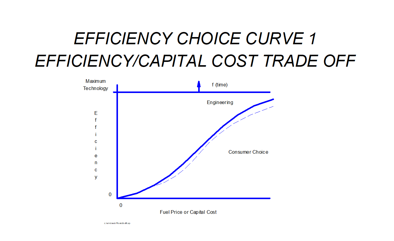
The default assumption for demand sectors in ENERGY 2100 is that both process and device efficiencies contain a trade off between the consumer selected efficiency (DEE/PEE) and capital costs. An efficiency curve is developed during the model’s calibration of input data that will generally result in higher capital costs as the selected level of efficiency increases at an increasing rate as we approach the assumed curve maximum efficiency. This is visually depicted in the following chart.
More detail about the efficiency curve methodology can be found the Volume 2 Demand Sector Structure Overview documentation. Specific to policies, there are several key components of curves to consider when developing an adjustment for efficiency:
- Moving up the efficiency curve (such as applying an efficiency standard) will produce higher capital costs and usually pass an increase in investments to an integrated macroeconomic model.
- Shifting the curve (done via adjusting PEMM/DEMM) will produce a higher level of efficiency at the same general cost point given the same fuel price.
- Capital costs can increase exponentially as we approach the maximum value without shifting the curve, which can produce very large and unrealistic investment values. Many policy files contain limits in place to avoid increasing efficiency to this level. This can be seen in these as a limit to keep a standard at most at 98% of the maximum value.